Transitioning to a new blog

 tl;dr: This blog will be following its sibling blog and transitioning to my personal site, blog.fixermark.com.

Changing to another blog engine

Effective today, new posts will be showing up at blog.fixermark.com instead of here. Blogger has been an excellent home for several years, but I've decided to shift my writing to my own server to simplify several things. Some details follow.

Why?

Several reasons, but the main ones are control and convenience. I've set up a pretty clean blog-authoring architecture behind the scenes using Hugo, and the most effort-intensive part next to "actually writing a blog post" is "reformatting the Hugo output to match to Blogger's requirements." Self-hosting just makes it easier to maintain the blog.

(... See that break in the background color there? The place where light cream gradient discontinuously jumps into flat orange? That's just a bug in the style of the theme Google provided. Can I fix it? Maybe. How? Don't know. On Hugo, I just set the background to a back-and-forth gradient and I'm happy).

Do you hate Google now?

Definitely not, in fact, I'm giving up several convenient features by going to self-hosting:

• The analytics here are top-notch, and the analytics I get on my own blog are far, far lower-resolution. I've chosen not to attach Google Analytics to my new blog as it brings concern for some readers, so such lack of resolution is to be expected.
• Google is very, ahem, generous with indexing blog posts on its own service into its index. In contrast, my personal blog has been off Blogger for several months now and has yet to show up in any search indices.
• Blogger's web interface works great. My new blog requires editing text files and uploading the results to a server.
• The new blog is totally statically-generated, so comments and timed publishing have to be done by me manually now. In contrast, this post went up automatically at the time I set it to.

All of that said: the driving factor to leaving is still UI convenience. Blogger's UI hasn't really evolved in ages, and for technical writing in particular it has some pretty severe friction points that I will not miss.

What of all the content that's already here?

Nothing will be deleted from this blog, because that would mess up way too many permalinks (and I'm not planning to put the effort in to clone all the articles here to the new site). You should be able to find everything here indefinitely.

So that's that then. Thanks for being my home for awhile Blogger; you did good work. But I'm hoping people enjoy the new blog, where I've already put up an article about building a plugin for the FIRST Robotics "Shuffleboard" dashboard program. Hope to see you there!

Where's Mark been?

 

So what happened to the rest of that drive train story?

Well, it's complicated. No literally. I dove into researching what I wanted to write next, and found it to be way more complicated than I thought. I'm digesting a bunch of control theory that has been too hard to fit into one blog post (for the record, mostly from this source). Once I can break off a piece worth sharing, I'll do so.

Wish me luck!

Simulating a differential drivetrain, part 1 - If it's stupid but it works...

There’s a lot going on in a drivetrain.

On the surface, they seem pretty simple: “Rotary power comes from somewhere. It’s moved through mechanical links. The links connect to wheels. Wheels make thing go.” But there’s a lot of subtle complexity that underpins all of that. Drivetrains can actually be one of the more complicated things to simulated on a robot.

In a FIRST competition, every robot has some method of getting around, so it’s worth the time to invest in learning how to simulat them and what is involved in simulating them. Over the next few weeks of posts, we’re going to dig deep on this topic. I’m going to start from a simple simulation, then move onto a more complicated one, and then finally onto one using built-in WPILib classes that tries to capture many, many details of the drivetrain. Along the way, we’ll compare the approaches and the results we get and see what the tradeoffs are.

Full disclosure: I’m as exploring as I am explaining here, dear reader. At the moment, I have only implemented one of these approaches before, so I don’t really know what we’ll discover. It’ll be exciting to see where we end up.

Before we start in with our first model, let’s talk a bit about what a differential drive is and what we’ll be comparing.

What’s a differential drive?

A differential drive (“diff drive”) is a drivetrain where the motors and wheels are divided into two independently controlled sets: left and right. By varying the power to each half, you can get the robot to move forward and backward or rotate (generally, for convenience, we want to build the robot so that point is in the middle of the chassis when the left and right trains are driven with equal but opposite inputs).

Since there’s no way for a diff drive to “sideslip”, we say diff drive is a non-holonomic system (which is a fancy way of saying there are paths through space an air-hockey puck could take but the robot can’t; it can’t move in an arbitrary direction while continuously spinning). But since the robot can turn on a dime, it should still be able to get everywhere (as opposed to a robot using car-style steering, which has some parking spots it can’t reach).

The simplest model of a differential drive is just two big wheels controlled by two motors, so that’s what we’re going to use. We’ll assume our wheels have a diameter of 4" (so about 0.1016 meters) so the robot goes about π * 0.1016 ≈ 0.3192 meters per revolution if both wheels are driven at the same speed.

The comparison

For each simulation, we’ll compare the following:

• Driving straight for three rotations (about one meter total, more precisely 95.76cm)
• Driving in a circle for three rotations (one motor full forward, one full back). Assuming a track width (distance between wheels) of 50 centimeters (about 19.6 inches), three wheel rotations are a distance along an arc of 31.92 centimeters in a circle with diameter 50 centimeters. Since the circumference of a circle is π * diameter, we can find the angle by

    length of arc / total circumference
  = 31.92 / π * 50
  ≈ 31.92 / 157.07
  ≈ 20.32% of the circle
  

  … which is about (2π * 20%) radians = 2/5π radians = 72 degrees.
• driving in a lazy arc (one motor full power, one motor half power) for three rotations. This one, I’m not going to lay out the math to predict what will happen yet (future post); we’ll just see what it does.

We’ll consider for each kind of simulator

• What results it gives us for our inputs
• How we set it up
• Velocity curves, acceleration curves, and final positions

And we’ll discuss some pros and cons.

Having established what we’re doing here, let’s start off with a very simple model.

The simple interpolator

So at first glance, the question of simulating a diff drive doesn’t feel too complicated. We know that

• If both motors go full-forward, the robot goes max-speed forward
• If both motors go full-backward, the robot goes max-speed backward
• If one motor is full forward and one full backward, the robot turns on a dime at max speed

The interpolation simulator just assumes that any motion the robot could be doing between these extremes is a simple linear interpolation of these motions. We establish a top speed for the wheel based on motor input (something simple, like “The robot goes at most 1 meter / second forward and rotates twice a second at max speed”). Then we split the motion in question into linear motion and turning motion.

• To figure out linear, we take the average of the sum of the left and right motor power and multiply that by top linear speed
• To figure out rotation, we take the average of the difference of the left and right motor (i.e. (left - right) / 2)) and multiply that by the top rotational speed

Then we update the robot’s speed and then update the robot’s position and heading based on that speed. Updating the position involves changing simulated encoder values, and updating the rotation involves changing a simulated gyro value.

There’s an implementation of this approach split between PoseEstimator.java and SimpleSimulatedChassis.java in this simulator demo.

Comparison and results

The end result feels okay; when hand-controlled; it’s not obviously broken. Here’s what it looks like on the tests of motion:

Note: one spot of trouble I got into testing this: you can change the refresh rate for graphs in Shuffleboard. If you set it too high, Shuffleboard becomes unresponseive and cannot edit the preference again. The fix is to delete the prefs from Java’s user prefs store (in my case, it’s stored in the system prefs in ~/.java/userPrefs/edu/api/first/shuffleboard/plugin/base/prefs.xml.

Linear motion

The “Drive” command (which causes the robot to drive forward until its encoder passes three rotations) causes the robot to drive forward and then stop; no problem. It gets pretty close to spot-on for the final value; the overage is likely due to the fact that the simulation happens in steps of 0.02 seconds; if the robot passes the target encoder rotation in one of those time steps, it can’t stop on a dime with simple on-off control and so stops a bit after the target.

The “Turn” command (which attempts to cause the robot to turn precisely 72 degrees) is similarly accurate. It also overshoots because turning can’t stop in the middle of a time step.

Worth noting is the acceleration and velocity result. Because the robot accelerates instantaneously, they are very spiky. This is unrealistic motion; real robots don’t immediately stair-step from zero velocity to some high velocity; they have to overcome inertia and static friction (and similarly, once moving, inertia will keep them moving and motors have to fight that to stop the machine). So our simulation isn’t particularly realistic.

Finally, we take a look at our lazy arc, which drives with the right motor full power and the left half power until we pass 72 degrees. The robot does trace a little arc, and we find our final position to be about a quarter-meter out in the x and y position with a heading of 76 degrees, closer to the 72-degree target than in raw turn (this makes sense; the rate of turn is lower on the lazy-turn mode).

Analysis

While this is good enough for practicing, it does not reflect how an actual robot behaves. For one thing, the motors cut on and off immediately, which doesn’t really reflect how motors work in the real world (see the discussion of the flywheel for details). For another, the robot’s path through space looks like a bunch of small line segments, since the facing is only allowed to update between steps and the robot always moves straight along its current facing. If the steps are small enough, this might be fine, but it doesn’t reflect well the curves that the robot actually travels in space.

Next week’s simulation approach will try to follow those curves.

Simulating a flywheel part 2: friction and time-step updates

On a previous post, I discussed creating a simulator for a simple flywheel in the FIRST Robotics WPILib framework in Java. We last discussed the high-level framework and simulating a motor; here, we’ll go into simulating friction and how we put it all together.

Friction is deceptively complicated

On the surface, friction is extremely simple. As is taught in high school physics, it’s the force that resists motion proportional to the normal force of the surface pushing against gravity. Which is to say, it’s just -K<sub>d</sub> * m * g, for g the gravitational constant (acceleration) and m the mass of the object, and K<sub>d</sub> the dynamic friction coefficient. Since the flywheel’s axle is pushed down by gravity on its socket, the friction force becomes a counter-torque opposing spin. So, no problem. We calculate the counter-torque, subtract it from the motor’s forward torque, and update every step. Punch that in and… Oh dear.

The problem is that friction is a continuous effect: the force opposing motion applies until the object gets very close to zero velocity (relative to the surface it’s rubbing against). At that point, the molecules of the two objects “gum up” with each other and the object stops moving. But the simulator is a discrete time-step simulation: every time step, the forces acting on the flywheel are summed up, velocity is changed, and then it’s assumed the flywheel velocity stays the same until the next time step. So the velocity “wiggles” back and forth around zero without ever reaching zero and the flywheel never actually stops.

There are several solutions of various levels of complexity for handling this aspect of friction, but for our purposes we can use a fairly simple one:

• Calculate the new angular velocity from the torques and counter-torques.
• Check to see if the sign of the velocity has flipped. If it has, we know the velocity crossed through the zero boundary.
• If we did cross zero, check to see if the driven torque exceeds the counter torque.
• If it doesn’t, the motor seizes; set velocity to zero.

Code as follows:

if (Math.signum(newAngularVelocityRps) != Math.signum(flywheelAngularVelocityRps)
    && flywheelAngularVelocityRps != 0
    && newAngularVelocityRps != 0) {
    // Crossed zero boundary; if torque is too low to overcome friction, motor seizes
    if (Math.abs(advantagedTorque) < Math.abs(counterTorque)) {
        newAngularVelocityRps = 0;
	}
}

One other aspect of friction to account for: Static friction generally exceeds dynamic friction, and applies if the flywheel is starting from zero velocity. We account for that by selecting the right friction coefficient based on whether the motor is moving and comparing the torque to the counter-torque from the friction; if driven torque does not exceed counter-torque, the motor doesn’t start.

var frictionCoefficient = m_motorSpeedRpm == 0 ?
          m_flywheelStaticFrictionConstant.getDouble(1.0) :
          m_flywheelDynamicFrictionConstant.getDouble(1.0);
// ...
var totalTorque = advantagedTorque - counterTorque;
if (m_motorSpeedRpm == 0 && Math.abs(advantagedTorque) < Math.abs(counterTorque)) {
    // stalled motor does not overcome static friction
    totalTorque = 0;
}

Putting it all together

Having accounted for friction, we now only need to take the total torques computed and apply them to how the velocity and encoder count changes over time.

To start, the total torque changes the angular velocity. Similar to the famous F = ma equation, torque = moment of inertia * angular acceleration. So we divide our torque by the moment of inertia to get an acceleration, and add it (times the time delta step) to the velocity:

var angularAccelerationRadsPerSec = totalTorque / m_flywheelMomentOfInertiaKgMSquared.getDouble(1.0);
var flywheelAngularVelocityRps = Units.rotationsPerMinuteToRadiansPerSecond(m_motorSpeedRpm) / gearRatio;

// Update angular velocity, parceling the change by the delta-T
var newAngularVelocityRps = flywheelAngularVelocityRps + angularAccelerationRadsPerSec * TIMESTEP_SECS;

Then, we just need to update the velocity and position for the encoder, and update the RPM graph:

m_motorSpeedRpm = Units.radiansPerSecondToRotationsPerMinute(newAngularVelocityRps * gearRatio);

// multiply by timestep and ratio of rotations to radians to get new flywheel position
var flywheelSpeedRotationsPerSec = newAngularVelocityRps / (2 * Math.PI);
var flywheelDelta = flywheelSpeedRotationsPerSec * TIMESTEP_SECS;

// encoder values are relative to flywheel, not motor
m_encoder.setDistance(m_encoder.getDistance() + flywheelDelta);
m_encoder.setRate(newAngularVelocityRps);

m_flywheelSpeedRpm.setDouble(flywheelSpeedRotationsPerSec * 60);

And we’re done! We have a self-updating flywheel simulation that we can experiment with.

Simulating a Flywheel part 1: overview and simulating a motor

Well, the off-season of FIRST Robotics is upon us. A time when young people’s minds turn away from robots and towards other things. Like simulating robots!

To give the team something to play with on the software side, I’m putting together a couple of simulators of robot subsystems to experiment with. The first one is a simple flywheel connected to one motor and encoder.

Interface for the simulator, showing the graph of flywheel RPM over time

I’m going to break the discussion of how I did this into two parts. Here, I’ll go over the top-level architecture of the program and how it tries to simulate, and talk about the equations to simulate a DC electric motor. In a follow-up post, I’ll go over the physics of friction simulation.

Full disclosure: I’m a rank amateur at this, putting together half-remembered high school physics, a barely-used robotics minor, and some hazy memories of graphs from my first years playing FIRST Robotics. Definitely room for improvement, and I welcome feedback on this.

You can get the simulator from the GitHub repsitory.

Overview

Program structure

The program is a simple TimedRobot operating at the default frequency of 50 times a second. It includes one automatically-running Flywheel subsystem that lets a motor be turned on and off (at max power or 0 power), which is controlled by a single joystick button.

In addition to Flywheel, a SimulatedFlywheel class is constructed if the robot is operating in simulation mode. This class takes in the motor from the Flywheel and a simulation wrapper around the encoder, allowing us to explicitly set the encoder’s position and velocity values.

The simulation

At a high level of abstraction, the torque on a motor-driven flywheel at any moment is simple:

Opposed forces acting on a spinning flywheel

Once we have calculated this torque, we can update the flywheel’s angular velocity by adding total torque / moment of inertia to the flywheel’s previous velocity. Then we update the flywheel’s position as well (accounting, in both cases, for the step of time over which this change is occurring, in our case 20ms between updates).

That’s the high-level approach; let’s drill down on the details.

Simulating motors

A DC motor is a relatively simple system, but it has a bit of complexity making simulating one interesting.

The basic principle by which a DC motor operates is that half of the motor uses electromagnets, while the other half uses permanent magnets. Varying the current through the motor’s electromagnets creates moving magnetic fields that the permanent magnets then “chase,” turning electricity into motion. The highest torque such a motor can give is when it’s “stalled” (i.e. not moving) and the voltage across it is maximized. At this configuration, the motor is pushing with its “stall torque” (note: It’s generally a bad idea to leave a motor stalled like this; many DC motors aren’t designed to run current through with no motion, and doing so for long periods of time can heat up and damage components).

So the total torque a motor can give is equal to some constant times the current through the motor:

Where I is current through the motor and k_M is a torque constant. Note: equations for motor behavior are mostly sourced from here. We can quickly calculate k_M as just the stall torque divided by the current, but for the purposes of the simulation i find it easier to just consider a relationship between stall torque and voltage by subsituting current through V = IR, then considering the motor with 12 volts across it and finding the value of a constant q which is resistance divided by K_M:

What’s interesting about electric motors is that when I say “some loops of wire acting as electromagnets near some permanent magnets,” I’m also describing a type of generator. And indeed, a spinning electric motor tries to induce a current in the direction opposite the spin! This opposing force, known as “back-EMF” (EMF: electromotive force), creates a counter-voltage to the voltage across the motor, resulting in a drop in current through the circuit. The physics of why this happens can be a little confusing, but there’s (I think) an elegant way to remember it: the fact that motors have back-EMF sort of falls naturally out of conservation of energy once we remember that motors with a voltage across them don’t spin up to infinite speed. Since a motor spinning at top speed only needs a little bit of energy to overcome resistance and maintain that speed, and since energy lost across a component of a circuit is the power (P=IV), we know that when the motor is spinning near top speed, P across the motor must be small to keep it spinning, so current and/or voltage diminished.

An electric motor and electric generator differ mostly in where the energy comes from. (Images sourced from Wikimedia)

The back-EMF on the motor is proportional to the motor’s rotational speed and some back-EMF constant k_e.

A motor allowed to spin up to full speed under no load and with maximum voltage across it will spin at a “free speed” which varies from motor to motor. At free speed, the back-EMF is approximately equal to the forward voltage, so we can set the voltage and speed in the above equation and re-arrange to solve for the back-EMF constant:

We’re closing in on simulating the torque. The remaining ingredient is the full torque equation.

To approach the final torque equation, we start by considering that the total voltage across the motor is the V=IR relationship through the motor plus the back-EMF value.

Substituting in the relationship between torque and current, we find

Now we have voltage, motor speed, and motor torque related. Doing the algebra to make torque the dependent variable and substituting our q constant for resistance divided by k_M, we get:

That gives us the motor torque in almost all circumstances, save one: what happens when the voltage is set to zero?

Brake or coast?

It’s a subtle bit of architecture, but an important one: as we’ve established, a motor acts like a generator. So what happens when the motor should be applying no power?

Motor controllers used in the FIRST Robotics competition are generally configurable to “brake” or “coast” mode. In “brake” mode, the controller short-circuits the motor to itself, allowing the back-EMF to try and drive the motor in reverse. This will resist motion in the motor and drag it to a halt much quicker. The mathematics of this is, honestly, something I don’t know.

“Coast” mode is much easier to model: in “coast” mode, the controller opens the circuit. With no ability for electricity to flow from one end of the motor to the other, the motor basically contributes no torque and the flywheel will spin down normally. So we special-case the zero-voltage condition to eliminate the motor torque, simulating “coast mode.”

Next steps

This gives us half the flywheel simulation. Next time, we’ll talk about the friction counter-torque (and how annoying friction subtleties are!) and tie it all together with the acceleration and velocity-update logic.

Piping Linux audio to a file

I recently had to pipe some audio from my browser to a file. This may not be the most elegant way, but I found it works.

Using SimpleScreenRecorder

For capturing audio and video, I use SimpleScreenRecoder. It’s a pretty no-frills recording program that is intended for (among other things) streaming content from a machine. While it supports both audio and video, I only care about the audio portion for this project.

To minimize bandwidth wasted recordin video, I set “Record a fixed rectangle” and set a 2x2 rectangle at 0,0. I then enabled “Record audio” with the PulseAudio backend and a Source of Monitor of sof-hda-dsp Speaker + Headphones. That output to my computer’s main speakers.

On the next screen, I set up an Output profile declaring the destination, use of MP4 as the container, an H.264 video codec with constant rate factor of 23, superfast preset, and “Allow frame skipping”, and an Audio codec of MP3, Bit-rate 128 kbit/s). 

Once set up, I could just start recording.

Resetting my monitor in Linux

Recently, I had an Ubuntu laptop I use regularly develop a weird quirk: sometimes when I plugged it into USB-C, neither the monitor nor power would connect. I discovered I could fix this by simply running lspci on the laptop, which somehow forced both to come back.

As this made no sense, I dug down a bit more. I can’t say I found an answer, but I did find some more things worth questioning.

PCI devices

On my laptop, devices are exposed at /sys/bus/pci/devices. Searching around a bit, I found that device /sys/bus/cpi/devices/0000:3b:00.0 was reporting itself as USB controller: Intel Corporation JHL6540 Thunderbolt 3 USB Controller (C step) [Alpine Ridge 4C 2016] (rev 02). Navigating into that subdirectory, I found I could sudo -s, then echo 1 > reset, which fixed the system in apparently the same way as running lspci.

What the hell?

At this point, I don’t really know. Sometimes the Linux architecture just puzzles me. I don’t know that lspci is running a reset on devices, but perhaps when it tries to poll details on the device, the act of polling itself trips a fault in the driver (becuase the driver realizes it can’t communicate with the device) and forces a reset to heal itself? I haven’t found any code confirming or falsifying this hypothesis; it’s still an open question for me.

On not giving up

Owning a Linux machine is like this. When things go wrong, the only person who’s responsible for fixing it is the owner. This is, ultimately, true of all self-owned computers, of course.

When I was younger, the ecosystem of Linux users was too hard to find to make this task easy; certainly not as easy as it was for Windows ownership, when everyone on the block had one of those machines. But the nice thing about living in the Internet era is Linux use bloomed, and at the same time users can find each other much more easily. I learned about the existence of the PCI list poking around on various sites.

There’s much more to learn, but it’s nice that resources are far easier to find now.

Visualizing access logs from my blog server

One of the things I’ve missed, having moved my blog off of Blogger, is the metrics. I don’t use the metrics for much, but there’s a nonzero serotonin hit to knowing that my content is read by someone. It’d be nice to be able to restore at least that piece of the Blogger feature-set.

Fortunately, I have access logs and a log analyzer.

I’ve settled on goaccess for my log analysis; it’s pretty straightforward, takes HTTP access logs as input, and presents the data visually (including on the command line). It’s installable on my local machine via the package manager (sudo apt-get install goaccess), so no problems there.

The steps are pretty straightforward:

• Get the logs
• Dump them into goaccess

The script to do that is short and sweet:

#!/bin/bash

SERVER=fixermark.com
LOGPATH=logs/personal-blog.fixermark.com/http
DESTINATION=logfiles

mkdir -p "$DESTINATION"
scp $SERVER:$LOGPATH/access.log* $DESTINATION
pushd $DESTINATION
# this is redundant because it's a symlink on the server to the most recent logfile
rm access.log.0
# gunzip will confirm replacing files
yes | gunzip -f *.gz
popd
goaccess $DESTINATION/access.log*

I run that, and I’m presented with a nice terminal interface for viewing the logs.

This is a good start!

Filtering

goaccess doesn’t support any filtering directly, but access logs are relatively simple to filter with command-line tools, and goaccess does support receiving its logs from the command line. Here’s a simple script to drop the logs related to various static content pieces:

cat $DESTINATION/access.log* | \
    grep -v /lib/ | \
    grep -v /css
	grep -v /images/ | \
    grep -v /js/ | \
    goaccess --log-format=COMBINED -

Adding this to the fetch script, the logs are now honed in on just posts.

To do next

Only a couple things I'd like to improve in this flow:

• scrubbing logs—after 21 days, I’d like to substitute the IP addresses with 0.0.0.0 to increase user anonymity.
• Run these server-side (or have goaccess pull them remotely, if possible) so logs aren’t living on more machines than strictly necessary.

Self Hosted Hugo Comments: data rendered with partials

In an earlier post, I added self-hosted static comments via shortcodes in Hugo. This approach had some benefits, but I didn’t like how it required modifying every blog page to support comments, even if no comments were present.

Hugo has a system of partials and templates to allow for similar pages to have the same layout. We can take advantage of these to handle comments on every blog page. This will pull the comments out of the main flow of the blog posts; we could move them into the front matter of the pages, but insted I’m going to knock out another con of the previous approach and consolidate all comments into one data file.

The method

We have a few steps to go through here:

• Consoolidate comments into a data file
• Build comments.html and comment.html as partials
• Build a new blogpost template to use the comments partial
• Use cascading front-matter to shift all the blog posts to the new template

Consolidate comments into a data file

To make it easy to work with comments as a separate construct from posts, we’ll shift all of them into a new file at data/comments.yaml. Hugo automatically parses files in the data directory and makes their content available for the site builder as site.data.<name of file>.

I’m using yaml because it splits the difference a bit: easy to use, but allows for multi-line strings without a lot of hassle (and it place nicely with my emacs config). here’s a snippet of the resulting yaml file.

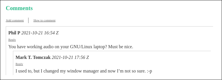
"/posts/2021/this-is-year-of-linux-on-desktop/":
  - id: 1
    username: "Anon 1"
    date: 2021-10-21T16:54:40.122Z
    comment: You have working audio on your GNU/Linux laptop?  Must be nice.
    replies:
      - id: 2
        username: Mark T. Tomczak
        date: 2021-10-21T17:56:00.084Z
        comment: I used to, but I changed my window manager and now I'm not so sure. :-p
"/posts/2021/marks-gallery-of-facebook-infractions-3/":
  - id: 1
    username: Anon-2
    date: 2021-06-14T15:34:10.877Z
    comment: |
      My vote is for "kill the filibuster." This is a failure of the algorithm to differentiate actual calls for violence from figurative language.  I wonder if you could post a comment about "Killing the Lights" when discussing what you might do before a movie or bedtime.

      Reminds me of when I tried to sell a dart board on FB Marketplace, and I included a photo of the darts themselves. I had my post removed for trying to sell weapons.

      There is an ENTIRE CATEGORY devoted to "Darts Equipment." Oh, Zuck...      

Worth noting:

• The top-level object is a dictionary mapping post paths to a list of the top-level comments in the posts
• comment IDs are unique within the post (they’re used to build URLs to email replies in)
• We preserved the tree structure from the previous short-code solution, but since the replies are now a separate field from the comment text body, we’ll be able ot use Markdown on the comment without mangling replies.

Build the comments.html partial

The partial at layouts/partials/comments.html finds the comments for the current page. If they exist, it stitches them in.

{{ with site.Data.comments }}
{{ $comments := index . $.Page.RelPermalink }}
<div class="comments">
  <h1 class="comments">Comments</h1>
  <div class="comments-menu">
    <ul>
      <li>
        <a href="mailto:blog+personal-comment@fixermark.com?body=Your Name:%0d%0aIcon:%0d%0aComment:&subject=Comment on {{ $.Page.Permalink }}">
          Add comment
        </a>
      </li>
      <li>
        <a href="/how-to-comment">How to comment</a>
      </li>
    </ul>
  </div>
  <div class="comments">
  {{ with $comments }}
    {{ $sorted := sort $comments "date" "desc"}}
    {{ range $sorted }}
      {{ partial "comment.html" (dict "comment" . "permalink" $.Page.Permalink) }}
    {{ end }}
  {{ else }}
      <div class="no-comments"><i>This article has no comments</i></div>
  {{ end }}
  </div>
</div>
{{ end }}

Once we fetch the list of comments, we check for any comment list with a key matching this page. If we find any, we sort them by date and render them ({{ range $sorted}}). This partial also renders a header for the comments section and a link to add a comment to the post.

Partials receive only the state given to them by their invoking template. When we render individual comments with the comment.html partial, we only give it the two pieces of information it needs (in the form of a new dictionary): the comment data as comment and the link to this page as permalink. The link is used to build replies to comments.

Build the comment.html partial

Rendering individual comments is delegated to a second partial.

<div class="comment">
  <div class="user-info">
    {{ if .comment.usericon }}
      <img src="{{.usericon}}">
    {{ end }}
    <span class="username">{{ .comment.username }}</span> <span class="post-time">{{ time.Format "2006-01-02 15:04 Z" .comment.date }}</span>
  </div>
  <div class="comments-menu"><a href="mailto:blog+personal-comment@fixermark.com?body=Your Name:%0d%0aIcon:%0d%0aComment:&subject=Comment on {{ .permalink }}?comment-id={{ .comment.id }}">Reply</a></div>
  <div class="comment-body">
    {{ .comment.comment | markdownify }}
  </div>
    {{ with .comment.replies }}
    <div class="replies">
      {{ $sorted := sort . "date" "desc" }}
      {{ range $sorted }}
        {{ partial "comment.html" (dict "comment" . "permalink" $.permalink) }}
      {{ end }}
    </div>
    {{ end }}
</div>

We pretty up the time representation of the comment using time.Format and run the body of the comment through markdownify to convert any special characters. We also add a reply link taking advantage of the comment ID.

Note that to render replies to this comment, this partial re-invokes itself passing the reply as the comment. This sort of recursion is fine in Hugo as long as it’s not infinite (the nature of the tree data structure this function is running on makes such infinite recursion impossible).

Build a new blogpost template to use the comments partial

Hugo allows pages to specify their type, which determines which of several templates Hugo will use to render the content of the page. Now that we have comments, I copied the single.html template from the theme I’m using into layouts/blogpost/single.md and replaced its invocation of a comment partial with my own:

{{ partial "comments.html" . }}

At this top level, I give the partial everything the template has for convenience.

Use cascading front-matter to shift all the blog posts to the new template

Hugo uses a speciall-named _index file to allow for application of front-matter to every page in a subdirectory of the site. Using that, it’s straightforward to shift all my blog posts to the new tepmlate. I add the file content/posts/index.md:

---
cascade:
  type: blogpost
---

Now, every page under posts/ has its type set by default.

Putting that all together (and adding a bit of CSS to clean the formatting), we now have comments on every page without changes to every page. Very happy with the result!

Pros and cons

Pros

Thread flow still clear

Replies are nested under their comments. I’m glad I didn’t have to lose this from the inline solution

Comment text is just markdown

I’m much happier with markdown as the comment body text than markup; easier to read, and modestly harder for end-users to find a way to accidentally break the whole sight flow

Cons

Comments no longer live on their articles

I’m considering this a pro in the overall assessment. It’d be nice if comments lived right next to their articles, but with comments consolidated in one file it’s much easier to manage them as an entity (including scrubbing one if a user asks to have it removed; I only have to purge one file through all archives).

Final thoughts

I’m really finding Hugo very straightforward to use. It’s nice to have my toolchain more tightly integrated and this level of control over both content and presentation.

Self Hosted Hugo Comments: embedded in page with shortcodes

Having chosen to self-host my Hugo comments as part of the static page content, there are a couple of ways to do it. In this article, I explore embedding them in the page using shortcodes.

The method

Comments in my blog are represented by two shortcodes.

comment.html

The first shortcode collects comment data in a semi-structured way and emits it as HTML. Here’s the whole thing.

/layouts/shortcodes/comment.html

{{- $postid := default (.Get 0) (.Get "id") -}}
{{- $username := default (.Get 1) (.Get "username") -}}
{{- $usericon := default (.Get 2) (.Get "usericon") -}}
{{- $postdate := default (.Get 3) (.Get "date") -}}

<div class="comment">
  <div class="user-info">
    {{ if $usericon }}
      <img src="{{$usericon}}">
    {{ end }}
    {{ $username }} {{ $postdate }}
  </div>
  <div class="comments-menu"><a href="mailto:blog+personal-comment@fixermark.com?body=Your Name:%0d%0aIcon:%0d%0aComment:&subject=Comment on {{ $.Page.Permalink }}?comment-id={{ $postid }}">Reply</a></div>
  <div class="comment-body">
    {{ .Inner }}
  </div>
</div>

This code is triggered as, for example,

\{\{< comment id="100" username="Phil P" date="2021-10-21T16:54:40.122Z" >}}
You have working audio on your GNU/Linux laptop?  Must be nice.

  \{\{< comment id="101" username="Mark T. Tomczak" date="2021-10-21T17:56:00.084Z" >}}
  I used to, but I changed my window manager and now I'm not so sure. :-p
  \{\{< / comment >}}
\{\{< / comment >}}

Note that the approach supports nesting; a comment emitted into the Inner material of another comment is just copied along with the other content, so we just roll the comment tree up as we go.

Also worth noting in the definition of the shortcode is the mailto link. The link is constructed such that it auto-populates the body and the subject for easy adherence to the commenting policy; uesrs get started with a template email that will get me the right information to add their comment. Right now, this process is manual, but I’ve attempted to wire it up so it can be easily automated in the future.

comments.html

A wrapper shortcode serves as an envelope for all the comments on the page and provides some placeholder text if there are no comments.

/layouts/shortcodes/comments.html

<div class="comments">
  <h1 class="comments">Comments</h1>
  <div class="comments-menu">
    <ul>
      <li>
        <a href="mailto:blog+personal-comment@fixermark.com?body=Your Name:%0d%0aIcon:%0d%0aComment:&subject=Comment on \{\{ $.Page.Permalink }}">
          Add comment
        </a>
      </li>
      <li>
        <a href="/how-to-comment">How to comment</a>
      </li>
    </ul>
  </div>
  \{\{ if (not .Inner) }}
  <i>This article has no comments</i>
  \{\{ else }}
  \{\{ .Inner }}
  \{\{ end }}
</div>

This code injects the HTML to show a Comments section in the page; it constructs a mailto link like the Reply button does (exercise for the reader: both of those links can stand to be further consolidated into their own shortcode, since they’re so similar). It also provides a simple placeholder text if there are not yet any comments.

Overall, I’m not at all unhappy with the result! (Editor’s note: I haven’t done a CSS pass on this yet, this just shows structure).

Pros and cons

Overall, I’m not unhappy with this approach, but it has some tradeoffs.

Pros

Thread flow is very clear

The fact replies are nested means it’s easy to see the flow of the conversation by reading the markdown itself.

Comment text is just markup

The comment text is just inline HTML, so relatively easy-to-read. It also supports everything I could possibly want to support (abuse of this—after all, it’s user-supplied content directly injected into the page—is moderated by the fact that the comments are hand-stitched into the page by me).

Cons

Mixes content and presentation

To support this approach, we need the \{\{< comments >}} shortcode on every page. Even though Hugo supports template pages (archetypes), that’s a maintenance burden. Ideally, stitching comments into the page should be the job of the layout itself, while the comments would be metadata for the page.

Markup, not markdown

Because shortcodes output HTML, I can’t use Markdown for the body of the comments; trying to pass a comment with replies through the Markdown parser mangles the HTML emitted by the nested \{\{< comment >}} shortcodes. Markdown is easier to work with and further constrains the styling in a nice way, which I enjoy.

Lack of consolidation

There’s benefit to having comments consolidated in one place for management. For example, adding a new comment with this approach requires mapping from the Subject line of an email to the relevant URL (and comment ID). If comments were consolidated in one place, adding new comments would be a simple append operation.

What’s next?

This approach is working for now, but I’m going to pursue moving the comments into page front-matter (or even a central data file that is read once and built into a scannable structure).

I'm switching my personal blog to self-hosting via Hugo

After putting a bit of thought into it, I’ve decided to start the process of switching my personal blog to self-hosting on Hugo instead of hosting through Blogger. This blog is staying where it is, but I’ve been playing with the Hugo framework for awhile and am finding I really enjoy it. Expect to see some posts about my experiences with it in here from time-to-time.

Why switch?

Even with the benefit of Google Takeout, moving blog infrastructure is time-consuming. So why have I bothered? A few reasons, in no particular order:

Tooling and control

Blogger’s UI hasn’t been updated in approximately ten years. It’s an acceptable WYSIWYG editor, but the resulting under-the-hood HTML is opinionated and has some weird formatting decisions. The editor also doesn’t support many keyboard accelerators, and it’s incredibly frustrating to have to break flow typing to go push a button to change style. In practice, I’ve been side-stepping the UI completely for weeks by writing blog posts in Markdown and copying-and-pasting the resulting HMTL directly into the raw editor view in Blogger. And I’m ultimately at the mercy of Blogger’s opinion of how layout should be done; some of my images overflow the content space, and I can either shrink them or leave that as-is.

Hugo lets me cut out the middle-man in that process; it renders directly from Markdown to HTML and the rendering can be reconfigured. The renderer is extensible via shortcodes that tap into the Go infrastructure under the hood. I’m doing most of my blogging in emacs now, and it feels great. In the future, I should be able to automate the flow of adding a post, recompiling, uploading to my server, and publishing updates.

Privacy, tracking, and censorship

Of all the reasons, this is the least significant one, but it bears mentioning: I think enough of my potential readers have come to care about the information-harvesting capacity of Google that I’d like to do them a solid and move off of a Google-hosted service. I’ll lose some of my analytics, and I have to support my own comments, but I think those are going to be exciting enough challenges to justify the cost. The recent rulings regarding Google Analytics and the GDPR seem to have some people backing towards the exits on that infrastructure anyway.

Google also has a bad habit (or good habit, if your goal is to combat spam and bad actors; I’m still enough of a company man that I see it their way too) of deciding you’ve violated their terms of service and blowing all your Google services out of the water as a result. I’ve already soft-firewalled the personal blog behind ownership by my non-primary account, but since it’s the “spicier” one, I run the risk that I’ll trip over Google’s constantly-evolving TOS some day, they’ll decide my primary and non-primary accounts are the same actor, and I’ll lose both. Moving the entire thing off to another host decreases the odds of that outcome.

Things I’ll miss

Not too many, it turns out.

Embedding images

One thing the WYSIWYG editor actually does do quite nicely is image embedding. The flow in Hugo isn’t as clean; I have to copy the image into a folder alongside the blog post and then reference the filename in the Markdown. That having been said, I strongly suspect I’ll be able to automate that process with a couple of emacs macros to turn it into fetching an arbitrary file, copying it into the right location, and adding the reference.

It turns out, embedding video is more straightforward in Hugo; there’s a shortcode for linking to YouTube (assuming I don’t just self-host the video content).

Will the old content be going away?

No. I don’t plan to add more posts to the personal blog, but I’ll be keeping it up so that hyperlinks don’t break. This will, in practice, fork comments, but I’ve decided I don’t care too much about that issue (comment load is low enough that it’s a non-issue).

How will you do comments on the new blog?

Great question! As a static site generator, Hugo’s engine doesn’t handle comments natively. Hugo integrates with a variety of comment engines, but after putting some thought into it and reading what others have done, I decided to just have people email me comments and I’ll embed them into the site. This doesn’t completely detach me from Google (my email service is GMail), but it gives users some confidence that I’m not dumping their information directly into the hopper.

Will I be moving this blog?

It’s possible, but I think unlikely in the near future. This one is heavier (including more images and more posts), and will take quite a bit more time. But if my experience with the personal blog goes well, we’ll see.

Where is the new blog?

The new blog is at http://personal-blog.fixermark.com. You can also subscribe to the Atom RSS feed.

Animating pulsing hexagons

Now that we can draw some hexagons, I'd like to animate them cross-fading occasionally from one color to another. This process will involve a few steps; we need to set up a rudimentary animation framework, and from there we'll take advantage of it to control the color of specific hexes and update them as they cross-fade back and forth.

The framework

The animation framework is pretty simple: * A HexAnimate abstract object to track animation state and update the canvas * A PulseHex concrete object that cross-fades a hex from one color to another and back * A list of currently-running animations * An update loop * A system for spawning new animations when the previous one is done

HexAnimate

A HexAnimate object is just an object that knows how to animate itself:

public abstract animate(timestamp: number, ctx: CanvasRenderingContext2D): boolean;

The timestamp is passed in so every animating element is sync'd to the same time, ctx is where to render to. Finally, the whole animate method returns true if it should be scheduled again next animation frame or false if it is done animating and can be discarded.

PulseHex

The PulseHex is a non-generalized animation to cross-fade one hex's color from a start point to a "peak" point and back over time.

export class PulseHex extends HexAnimate {
    constructor(
        private xIndex: number,
        private yIndex: number,
        private startTime: number,
        private peakTime: number,
        private endTime: number,
        private startColor: Color,
        private endColor: Color) {
        super();
    }

    public animate(timestamp: number, ctx: CanvasRenderingContext2D): boolean {
        if (timestamp > this.endTime) {
            // Render one last time to clear all the way to the initial color
            ctx.save();
            HEX_TEMPLATE.offsetToHex(ctx, this.xIndex, this.yIndex);
            HEX_TEMPLATE.render(ctx, colorToCode(this.startColor));
            ctx.restore();

            return false;
        }
        const color = timestamp < this.peakTime ?
            interpolate(this.startColor, this.endColor, (timestamp - this.startTime) / (this.peakTime - this.startTime)) :
            interpolate(this.startColor, this.endColor, (this.endTime - timestamp) / (this.endTime - this.peakTime));


        let stringRep = colorToCode(color);

        ctx.save();
        HEX_TEMPLATE.offsetToHex(ctx, this.xIndex, this.yIndex);
        HEX_TEMPLATE.render(ctx, stringRep);
        ctx.restore();

        return true;
    }
}

The constructor takes in the X and Y index of what hex to animate, a start, peak, and end timestamp, and what color we should start (and end) at and the color we should reach at peak time.

The animation logic splits into a terminator and a continuation: the first condition checks to see if we're past end time, and if we are we draw one last hexagon at start color to reset the hex to initial conditions. If we're not, we pick a color by interpolating between start and end (if before peak time) or end and start (if after peak time). The interpolation function is a very simple a + t(b-a) interpolation of each of the red, green, and blue components; not the fanciest (or necessarily the best-looking from a human perception standpoint), but it's a reasonable starting point. Once color is chosen, we draw the relevant hexagon.

List of currently-running animations

let animations: HexAnimate[] = [];

Nothing fancy here; literally an array of animation objects. Worth noting is that this allows more than one to be running at a time; we don't take advantage of that right now, but we will!

Update loop

const timestamp = Date.now();

// ...

animations = animations.filter((animation) => animation.animate(timestamp, context));

updateBackground(canvas);

setTimeout(updateRender, 1000 / FPS);

The update loop is very simple: we ask every animation to run, and if it returns false we drop it out of the list of animations for next loop. Once they've run, we push the new canvas to the background and schedule ourselves to run again.

A system for spawning new animations when the previous one is done

if (animations.length === 0) {
    animations.push(new PulseHex(
        Math.floor(Math.random() * (CANVAS_HEXES_ACROSS - 2)) + 1,
        Math.floor(Math.random() * (CANVAS_HEXES_DOWN - 2)) + 1,
        timestamp,
        timestamp + 1000,
        timestamp + 3000,
        codeToColor(DEFAULT_HEX_COLOR)!,
        {
            r: Math.random() * 256,
            g: Math.random() * 256,
            b: Math.random() * 256,
        }
    ));
}

When our animation queue is empty, we construct a new one. This approach will guarantee us exactly one running at all times. We cheat a bit on the logic of the X and Y coordinates to inset from the edges so that we don't reveal the repetition seam of the background image.

With all those pieces put together, I'm pretty happy with the end result!

The full code is available on GitHub.

XMonad: giving a window affinity to live on a given workspace

I've been working on a project (http://usfirst.org) that combines vscode with a simulator to run Java locally. One small annoyance is that every time the program runs, the simulator opens a new window on the same desktop, but it's intended to be run full-screen. Since I'm running XMonad, I have to manually window-shift-number to send the simulator off to another workspace. That's the sort of annoyance I run my own window manager to deal with.

So let's deal with it.

First, we have to discriminate the simulator window from others. No major issue there; the xprop command-line tool lets us get details on the window. Just run and click.

> xprop
  WM_STATE(WM_STATE):
        window state: Normal
        icon window: 0x0
  _NET_WM_ICON_NAME(UTF8_STRING) = "Robot Simulation"
  _NET_WM_NAME(UTF8_STRING) = "Robot Simulation"
  WM_LOCALE_NAME(STRING) = "en_US.UTF-8"
  WM_CLIENT_MACHINE(STRING) = "rambler"
  WM_ICON_NAME(STRING) = "Robot Simulation"
  WM_NAME(STRING) = "Robot Simulation"
  XdndAware(ATOM) = BITMAP
  WM_CLASS(STRING) = "Robot Simulation", "Robot Simulation"
  WM_NORMAL_HINTS(WM_SIZE_HINTS):
        program specified location: 0, 0
        window gravity: Static
  WM_HINTS(WM_HINTS):
        Initial state is Normal State.
  _NET_WM_PID(CARDINAL) = 14024
  WM_PROTOCOLS(ATOM): protocols  WM_DELETE_WINDOW, _NET_WM_PING

The relevant detail here is WM_CLASS, which is the window class and appears to be the nice, stable string "Robot Simulation". Great!

XMonad includes manageHook rules that let us hook into the rules for window config. Documentation lives here; there's a lot, but the most relevant ones are that we can get the class of the window (className) and we can direct the window to go to a different workspace (doShift). The stanza is a simple piece of XMonad line noise:

windowAffinities = className =? "Robot Simulation" --> doShift "9"

... then just modify the top of my xmonad declaration to include that logic.

main = do
    xmproc <- spawnPipe "xmobar"

xmonad $ docks defaultConfig
     { manageHook = windowAffinities <+> manageDocks <+> manageHook defaultConfig

(Note: if you want more than one, the composeAll [ hooks ] grouping will do so. Just make sure the brackets [] get on their own lines, or Haskell will complain "parse error (possibly incorrect indentation or mismatched brackets)".

Added that stanza, a quick Windows-Q to reload the XMonad rules, and the next time the simulator opened, it opened on workspace 9. Just a little less typing to do what I mean.

Tilted hexes with CSS

Now that we can render and animate hexagons, can we tilt them?

Spoiler: yes

Directly in the rendering logic, this is tricky. I'll have to add a rotation to the canvas (easy) and then find the height and width of a rectangle overlapping the canvas at which tesselation occurs so I can tile the background (much less easy). Fortunately, CSS transforms can make this much easier—not perfectly easy, but not bad.

The big challenge doing something like this with CSS is that CSS conflates rendering logic and layout logic: every object visible on the page is a DOM element, and every DOM element impacts the page layout. In an ideal world, I could just set a rendering rule for the background and let layout operate separately (the element background-image type supported by Firefox gets close to allowing this). Instead, the approach is a bit more complex:

• Leave the background of body unchanged
• As children of body, have two divs: one to serve as background container, one to hold content
• The background-container div addresses the layout concern: it is set to fill 100% of the window and uses overflow: clip to clip off any excess content that tries to overflow the window
• As child of background-container, a background div is set larger than the window, is set to repeat its image, has the rotation applied, and has a z-index set to be behind other content
• The content div is set to also take up the whole window and has a z-index set to be in front of the background.

Without the background-container, the background forces the layout algorithm to try and fit the entire tilted element, which introduces unwanted scrolling.

It's not the prettiest CSS but it gets the job done.

.background-container {
    position: absolute;
    left: 0px;
    top: 0px;
    right: 0px;
    bottom: 0px;
    overflow: clip;
}
#background {
    position: absolute;
    left: -100%;
    top: -100%;
    right: -100%;
    bottom: -100%;
    background-repeat: repeat;
    transform: rotate(-20deg);
    z-index: 0;
}

.content {
    position: absolute;
    left: 0px;
    top: 0px;
    right: 0px;
    bottom: 0px;
    z-index: 1;
}

And the result is pretty satisfying!

Animating a web page background

Having confirmed that I can dynamically generate a web page background by rendering an image to canvas (and then setting that canvas's data URL as the background CSS value), the next question becomes: can I animate it?

The cheapest way to do that is with setTimeout. This isn't ideal (it'll block on the UI thread), but does it work at all?

The answer is yes!

The code for the demo is relatively straightforward.

const SEGMENT = 100 / 6;
const HEX_HEIGHT_WIDTH_RATIO = 1.1547005;

const MAX_VALUE=0xdd;

const FPS = 24;

let curTime = 0;
let currentValue = 0;
let ascending = true;

function renderBg(color: string) {
    const canvas = document.createElement('canvas');
    canvas.width = 100;
    const HEIGHT = SEGMENT * 4 / HEX_HEIGHT_WIDTH_RATIO;
    canvas.height = HEIGHT;
    const ctx = canvas.getContext('2d');
    if (!ctx) {
        return;
    }

    ctx.fillStyle = '#' + color;
    ctx.fillRect(0,0,100,HEIGHT);


    ctx.strokeStyle= "white";
    ctx.lineWidth = 3;
    ctx.beginPath();
    ctx.moveTo(0, HEIGHT / 2);
    ctx.lineTo(SEGMENT, HEIGHT / 2);
    ctx.lineTo(2 * SEGMENT, 0);
    ctx.lineTo(4 * SEGMENT, 0);
    ctx.lineTo(5 * SEGMENT, HEIGHT / 2);
    ctx.lineTo(100, HEIGHT / 2);
    ctx.moveTo(SEGMENT, HEIGHT / 2);
    ctx.lineTo(2 * SEGMENT, HEIGHT);
    ctx.lineTo(4 * SEGMENT, HEIGHT);
    ctx.lineTo(5 * SEGMENT, HEIGHT / 2);
    ctx.stroke();

    const body = document.getElementsByTagName('body').item(0);
    if (!body) {
        return;
    }
    body.style.background=`url(${canvas.toDataURL()})`;
}

function updateRender() {
    let increment = (MAX_VALUE / 2.0 / FPS);
    if(!ascending) {
        increment = -increment;
    }

    currentValue += increment;
    if (currentValue > MAX_VALUE || currentValue < 0) {
        currentValue = Math.min(MAX_VALUE, Math.max(0, currentValue));
        ascending = !ascending;
    }

    let stringRep = Math.floor(currentValue).toString(16);
    while (stringRep.length < 2) {
        stringRep = '0' + stringRep;
    }

    renderBg(`EEEE${stringRep}`);

    setTimeout(updateRender, 1000/FPS);
}

setTimeout(updateRender, 1000/FPS);

The approach is pretty straigtforward: run a function 24 times a second to cycle through colors and redraw the background, then output the updated background data-URL to the body's background CSS property.

Performance isn't perfect (GPU process eats about 24% of my CPU when the tab is foreground), but the UI thread doesn't appear to be badly blocked. I'll have to test it on mobile next to see how much it harms performance.

Dynamic web page background with the Paint API

To spruce up the look of Swătch, I'm investigating animating a background for the game. This turns out to be a bit less trivial than I'd hoped; there are a couple of options, but none of them at this time are great. In this post, I'll describe some options I considered and which I settled on.

The bestagon

CSS Painting API

A relatively new proposal is the CSS Painting API. This API lets you "hook" the CSS rendering pipeline via code similar to a web-worker. When CSS demands an image to render, it will delegate to your painter with a 2D render context, height and width of the space to draw, and any additional CSS properties you declare that your painter receives; you then render into the provided context (using JavaScript code) and CSS will use the result as an image.

This API is powerful, but hooking into it required some adjustment. To build a web worker, I had to modify my webpack configuration to emit two output files; webpack supports this via modifying the entrypoint to use object syntax and then modifying the output rule to look like [name].js to template-in the object name from the entrypoints. But I then had to fight TypeScript because the Painting API isn't in the dom types yet; I fought with webpack trying to use .d.ts files (tricky; webpack hates this) but finally gave up and wrote the paint worker in plain ol' JavaScript.

Pros:

• Anything you can do in canvas rendering (kinda) you can do to the background of your object
• Uses regular CSS, so tools like animations work

Cons:

• Fighting with TypeScript to use an API that isn't typed yet
• Modify webpack to emit a web worker
• (the big one) This API not supported by Firefox of Safari yet

Deciding I didn't want to limit my new feature to only Chrome users, I sought an alternative.

toDataURL and canvas

It's possible to have a bare canvas object emit its image buffer via a data URL. Once you've done that, you can set the background image of an element to that data URL, and you're all set. A bit inefficient, but it works. There's a great tutorial post here describing the process.

Armed with this approach, it was relatively straightforward to build a small hexagon background on a 100 x (height of the hexagon) rectangle.

Pros:

• Supported in all modern browsers
• Works with background-repeat CSS, so constructing and setting a small image automatically gives you tesselation

Cons:

• Will this be fast enough to do simple animations? Not yet sure

Armed with this approach, I put together a simple demo on top of my testbench to prove out the idea.

index.ts:

const SEGMENT = 100 / 6;
const HEX_HEIGHT_WIDTH_RATIO = 1.1547005;

function go() {
    const canvas = document.createElement('canvas');
    canvas.width = 100;
    const HEIGHT = SEGMENT * 4 / HEX_HEIGHT_WIDTH_RATIO;
    canvas.height = HEIGHT;
    const ctx = canvas.getContext('2d');
    if (!ctx) {
        return;
    }

    ctx.fillStyle = '#EEEEDD';
    ctx.fillRect(0,0,100,HEIGHT);


    ctx.strokeStyle= "white";
    ctx.lineWidth = 3;
    ctx.beginPath();
    ctx.moveTo(0, HEIGHT / 2);
    ctx.lineTo(SEGMENT, HEIGHT / 2);
    ctx.lineTo(2 * SEGMENT, 0);
    ctx.lineTo(4 * SEGMENT, 0);
    ctx.lineTo(5 * SEGMENT, HEIGHT / 2);
    ctx.lineTo(100, HEIGHT / 2);
    ctx.moveTo(SEGMENT, HEIGHT / 2);
    ctx.lineTo(2 * SEGMENT, HEIGHT);
    ctx.lineTo(4 * SEGMENT, HEIGHT);
    ctx.lineTo(5 * SEGMENT, HEIGHT / 2);
    ctx.stroke();

    const body = document.getElementsByTagName('body').item(0);
    if (!body) {
        return;
    }
    body.style.background=`url(${canvas.toDataURL()})`;
}

go();

The result generated the pattern at the top of this post; I'm not at all unhappy with it!

Setting up a test bench for TypeScript compiled client code with Node.js (why are things like this?)

My first computer was an Apple ][c owned by my parents. In that environment, booting the machine with no disk in the drive would load a working development environment in the form of an Applesoft BASIC REPL.

Sometimes, when I spend an hour configuring a development environment for testing a web application, I miss those days.

I've uploaded a bare-bones testbench to GitHub for playing with TypeScript code compiled to run in a browser client. To do so, I set up the following dependencies:

• typescript
• webpack (collects JavaScript into one file)
• ts-loader (lets webpack drive TypeScript compilation)
• webpack-cli (command-line tools to drive webpack)
• webpack-dev-server (server to watch system changes)

Once these were installed, I had to set up with a tsconfig.json file for TypeScript and a webpack.config.js file for webpack. It took a little while to pull all the pieces together, but the nice thing is that now they're set up and I don't have to do it again.

Why are things like this?

When I look back on how programming was when I started vs. now, I get nostalgic from time-to-time about how things were simpler. We just turned the computer on and coded it! What happened?

More flexibility means more complexity

The computer I coded on when I was six did exactly one thing at a time. Meanwhile, as I type this, I have my testbench open in another window, documentation for npm in a second window, my blog statistics open in a third window... Modern computers are simply more flexible, and there does exist a strong correlation between flexibility and complexity.

In a real sense, the art of software engineering isn't creating features, it's denying options. The most featureful computer is a machine exposing a REPL. You can do anything it can do! You just have to write the code! But we've built an entire global industry around paring down the set of possible things a computer could do to the subset people actually want to do (and in so doing, surfacing those features behind a few buttons at the cost of pushing every other feature of the machine deeper into a tree of options). An Apple ][c with no disk in it "knew" I wanted to program something in BASIC when I turned it on; a modern computer has no "idea" what the user wants.

Since building a tiny web server with TypeScript and Node.js is as likely to be what I want to do as checking my bank account, there is necessarily more complexity to make it happen.

Embedded development isn't like desktop development

Since I'm working on "just some browser stuff," it's easy to fall into the trap of thinking that what I'm doing is simple. Browsers are easy to code; pop open one text file and start writing.

That's true... If you want to code in HTML and JavaScript. But add TypeScript to the mix and, oops, I'm not doing "native" coding anymore. Now I need an infrastructure to deal with the impedance mismatch between the fact that the browser only understands JavaScript and HTML and the fact that the only context I'm willing to code in bare JavaScript anymore is if a child's life is on the line (and even then, it'd better be a child I like).

Looked at in this way, writing web comtent in TypeScript isn't even just compiled; it's more like embedded development: we are writing code in a language not directly supported by the embedding target (the browser) and we need to update the target's view of the code when it changes (recompile and put the data where the browser can see it). In that sense, writing web content with TypeScript looks a lot more like writing code against a microcontroller (albeit a fancy microcontroller run in a virtual machine on my desktop) than writing a BASIC program. Some complexity is to be expected. 100% of the dependencies I installed were to support automatic recompilation and hosting of changes to the code without having to stop and re-start a server.

The real problem is discoverability

At the end of the day, none of these problems would be problems if I already knew what I was doing. This testbench isn't the first one people have written (nor will it be the last). But currently, a search on GitHub for typescript node testbench only returns my code repository!

This can't be true.

I can hope that someone sees this blog post and that the existence of my project somehow gets into StackOverflow or Google search results, but ultimately, this is the real complexity of modern programming: when you want to do something relatively simple, how do you get started? In the '80s, I could start by powering on the computer. How do I start now? typescript node getting started returns several more results, but none quite what I'd want (most of them add more complexity than I need; many are descriptions of how to solve the problem, not workable starter code).

This problem isn't trivial to solve; computing moves fast these days. Several of the technologies I'm using for this project didn't exist ten years ago. But putting starter frameworks in a place people can find them (and perhaps, even, creating a language where people can describe what they want) still feels like a problem in need of a better solution.

We've made incredibly flexible machines, and our ability to talk about them hasn't caught up to the inherent complexity of that flexibility.