Simulating a differential drivetrain, part 1 - If it's stupid but it works...

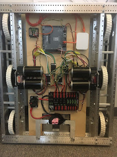
There’s a lot going on in a drivetrain.

On the surface, they seem pretty simple: “Rotary power comes from somewhere. It’s moved through mechanical links. The links connect to wheels. Wheels make thing go.” But there’s a lot of subtle complexity that underpins all of that. Drivetrains can actually be one of the more complicated things to simulated on a robot.

In a FIRST competition, every robot has some method of getting around, so it’s worth the time to invest in learning how to simulat them and what is involved in simulating them. Over the next few weeks of posts, we’re going to dig deep on this topic. I’m going to start from a simple simulation, then move onto a more complicated one, and then finally onto one using built-in WPILib classes that tries to capture many, many details of the drivetrain. Along the way, we’ll compare the approaches and the results we get and see what the tradeoffs are.

Full disclosure: I’m as exploring as I am explaining here, dear reader. At the moment, I have only implemented one of these approaches before, so I don’t really know what we’ll discover. It’ll be exciting to see where we end up.

Before we start in with our first model, let’s talk a bit about what a differential drive is and what we’ll be comparing.

What’s a differential drive?

A differential drive (“diff drive”) is a drivetrain where the motors and wheels are divided into two independently controlled sets: left and right. By varying the power to each half, you can get the robot to move forward and backward or rotate (generally, for convenience, we want to build the robot so that point is in the middle of the chassis when the left and right trains are driven with equal but opposite inputs).

Since there’s no way for a diff drive to “sideslip”, we say diff drive is a non-holonomic system (which is a fancy way of saying there are paths through space an air-hockey puck could take but the robot can’t; it can’t move in an arbitrary direction while continuously spinning). But since the robot can turn on a dime, it should still be able to get everywhere (as opposed to a robot using car-style steering, which has some parking spots it can’t reach).

The simplest model of a differential drive is just two big wheels controlled by two motors, so that’s what we’re going to use. We’ll assume our wheels have a diameter of 4" (so about 0.1016 meters) so the robot goes about π * 0.1016 ≈ 0.3192 meters per revolution if both wheels are driven at the same speed.

The comparison

For each simulation, we’ll compare the following:

• Driving straight for three rotations (about one meter total, more precisely 95.76cm)
• Driving in a circle for three rotations (one motor full forward, one full back). Assuming a track width (distance between wheels) of 50 centimeters (about 19.6 inches), three wheel rotations are a distance along an arc of 31.92 centimeters in a circle with diameter 50 centimeters. Since the circumference of a circle is π * diameter, we can find the angle by

    length of arc / total circumference
  = 31.92 / π * 50
  ≈ 31.92 / 157.07
  ≈ 20.32% of the circle
  

  … which is about (2π * 20%) radians = 2/5π radians = 72 degrees.
• driving in a lazy arc (one motor full power, one motor half power) for three rotations. This one, I’m not going to lay out the math to predict what will happen yet (future post); we’ll just see what it does.

We’ll consider for each kind of simulator

• What results it gives us for our inputs
• How we set it up
• Velocity curves, acceleration curves, and final positions

And we’ll discuss some pros and cons.

Having established what we’re doing here, let’s start off with a very simple model.

The simple interpolator

So at first glance, the question of simulating a diff drive doesn’t feel too complicated. We know that

• If both motors go full-forward, the robot goes max-speed forward
• If both motors go full-backward, the robot goes max-speed backward
• If one motor is full forward and one full backward, the robot turns on a dime at max speed

The interpolation simulator just assumes that any motion the robot could be doing between these extremes is a simple linear interpolation of these motions. We establish a top speed for the wheel based on motor input (something simple, like “The robot goes at most 1 meter / second forward and rotates twice a second at max speed”). Then we split the motion in question into linear motion and turning motion.

• To figure out linear, we take the average of the sum of the left and right motor power and multiply that by top linear speed
• To figure out rotation, we take the average of the difference of the left and right motor (i.e. (left - right) / 2)) and multiply that by the top rotational speed

Then we update the robot’s speed and then update the robot’s position and heading based on that speed. Updating the position involves changing simulated encoder values, and updating the rotation involves changing a simulated gyro value.

There’s an implementation of this approach split between PoseEstimator.java and SimpleSimulatedChassis.java in this simulator demo.

Comparison and results

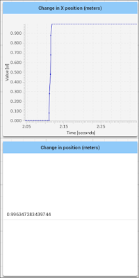
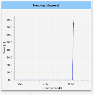
The end result feels okay; when hand-controlled; it’s not obviously broken. Here’s what it looks like on the tests of motion:

Note: one spot of trouble I got into testing this: you can change the refresh rate for graphs in Shuffleboard. If you set it too high, Shuffleboard becomes unresponseive and cannot edit the preference again. The fix is to delete the prefs from Java’s user prefs store (in my case, it’s stored in the system prefs in ~/.java/userPrefs/edu/api/first/shuffleboard/plugin/base/prefs.xml.

Linear motion

The “Drive” command (which causes the robot to drive forward until its encoder passes three rotations) causes the robot to drive forward and then stop; no problem. It gets pretty close to spot-on for the final value; the overage is likely due to the fact that the simulation happens in steps of 0.02 seconds; if the robot passes the target encoder rotation in one of those time steps, it can’t stop on a dime with simple on-off control and so stops a bit after the target.

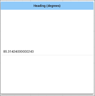
The “Turn” command (which attempts to cause the robot to turn precisely 72 degrees) is similarly accurate. It also overshoots because turning can’t stop in the middle of a time step.

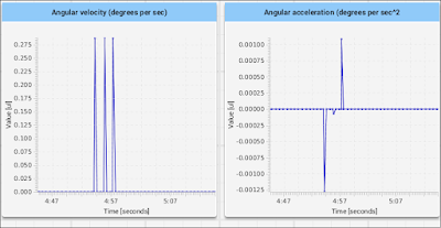
Worth noting is the acceleration and velocity result. Because the robot accelerates instantaneously, they are very spiky. This is unrealistic motion; real robots don’t immediately stair-step from zero velocity to some high velocity; they have to overcome inertia and static friction (and similarly, once moving, inertia will keep them moving and motors have to fight that to stop the machine). So our simulation isn’t particularly realistic.

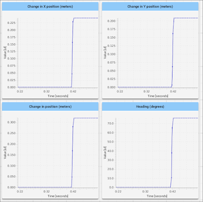
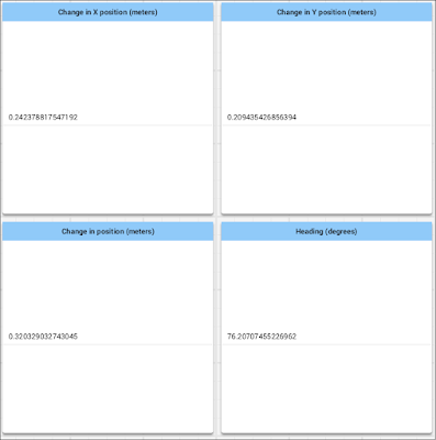
Finally, we take a look at our lazy arc, which drives with the right motor full power and the left half power until we pass 72 degrees. The robot does trace a little arc, and we find our final position to be about a quarter-meter out in the x and y position with a heading of 76 degrees, closer to the 72-degree target than in raw turn (this makes sense; the rate of turn is lower on the lazy-turn mode).

Analysis

While this is good enough for practicing, it does not reflect how an actual robot behaves. For one thing, the motors cut on and off immediately, which doesn’t really reflect how motors work in the real world (see the discussion of the flywheel for details). For another, the robot’s path through space looks like a bunch of small line segments, since the facing is only allowed to update between steps and the robot always moves straight along its current facing. If the steps are small enough, this might be fine, but it doesn’t reflect well the curves that the robot actually travels in space.

Next week’s simulation approach will try to follow those curves.